IN-Site Blog Post #1

Empirical Mean and Central Limit Theorem (CLT)

Note 0: If you are new to CLT or read it a while back, I would recommend watching the following video by Khan Academy and then resume reading thereafter.

This post is NOT about the proof but an application of CLT. I have heard of and used CLT in many problems but never “felt” it. I always figured it isn’t the hardest thing in the world as most people understand it in their first or second attempt. But somehow, I found it hard to wrap my head around this. It turns out that its role is significant in understanding of optimization in Machine Learning (ML). And so, I spent some time and finally “felt” it. This post is about the insight that I got.

I assume that the reader is familiar with the general setup of a supervised ML optimization problem. We observe some data \((X,Y)\) where capital letters denote they are random variables. Let’s group them together in a random variable \(Z=[X;Y]\) (MATLAB notation, more of a slang). We want to minimize the true expected loss, \(E[L(Z,\theta)]\) which will be a function of only \(\theta\), say \(f(\theta)\), where \(\theta\) are the (deterministic) parameters of the ML model.

First, why do we do this?

Because this \(L\) is a function of a random variable \(Z\) and hence a random variable itself. The best we can do, in minimization of any random quantity, is to minimize its expected value. Hence we minimize \(E[L]\) where expectation is over the probability density function (pdf) of random variable \(Z\) or equivalently the joint pdf of \((X,Y)\). Furthermore, we need to minimize the true \(E[L]\) but what we can practically get is a finite set of samples and hence, can only evaluate the sample/empirical mean, \(\hat{E}[L]=\frac{1}{n}\sum_{i=1}^n l_i\), where \(n\) is the no. of samples and \(l_i\) refers to the value of \(L\) for \(i^{th}\) data point (refer to this for more details). Now here is where the CLT starts to come in. We can intuitively feel that if we were given infinite or all possible samples of \(L\), we could evaluate the true mean \(E[L]\). But because we need to work with the finite empirical mean, is it even a good approximation of the true mean?

The essential part is to realize that this empirical mean is itself a random variable (say \(B=\hat{E}[L]\)) because it’s just a scaled sum of random variables \(Z\). But what is the pdf of \(B\). CLT tells us that for large enough no. of samples, \(n\), \(B \sim \mathcal{N}(\mu,\sigma^2)\) .

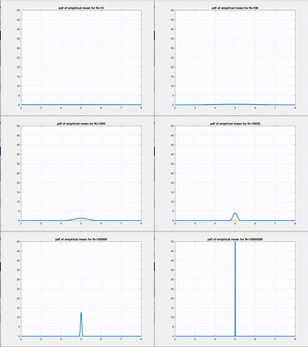
There it is! The empirical mean we calculate for any given dataset is nothing but a point sampled from a gaussian distribution whose mean \(\mu\) is the true mean \(E[L]\) we are seeking and variance \(\sigma^2\) is \(\frac{var(L)}{n}\). So, according to CLT, as n increases, this is what starts happening to the pdf of \(B\).

Clearly, the variance of the gaussian reduces and the pdf converges to a \(\delta(B-E[L])\) function as \(n\to\infty\). This figure is the pictorial representation of a more general phenomenon which we all have heard about, the convergence. So, empirical mean is just a point from this pdf. Therefore, as we can say for any sample from a gaussian pdf, we are 99% confident that this one point we sampled (empirical mean of a given dataset) is within \(\pm3\sigma\) of the true value we were seeking in the first place. Hence, the variance refers to the error in our estimate.

The bound can then be written as

\[P(|B-E[L]|\leq3\sqrt{\frac{var(L)}{n}})>0.9973\]

Note 1: Same concept can be extended to the gradient estimate after exchanging the order of application of the gradient and the expectation operator (due to linearity of both operators), i.e.

\(\nabla_{\theta}E[L]=E[\nabla_{\theta}L]=E[G(Z,\theta)]\) where point-wise gradient \(G\) is just another function like \(L\) and same things apply while calculating empirical expectations of gradients, whether on a batch or a mini-batch.

Note 2: This is a very basic perspective to the convergence question using CLT. There has been !A LOT! of research and proofs that follow, using advanced concepts/theorems which give better bounds. But this can be considered as a first step (I guess) towards that theory.

Hope this will help somebody, somewhere, someday.

-Tushar